Methodology

Read to understand how we calculate the overall Games' scores based on user submissions.

MyGameDNA scores games using two profiles: Challenge (skills needed to succeed) and Reward (satisfaction gained from succeeding). Each profile has Micro (reflexes/precision), Macro (planning/resources), and Mystiko (prediction/deduction), totaling 100%.

Three methods calculate the result: Method 1 prioritizes trusted experts, especially with few submissions; Method 2 (iForest) removes globally unusual submissions; Method 3 (LoOP) detects submissions that are unusual compared with nearby players. Finally, BHPCM combines all three, accounting for uncertainty and disagreement rather than simply averaging them, producing the final 100-point profile.

Challenge vs. Reward

Every game receives two independent profiles. Each profile is scored across three dimensions — Micro, Macro, and Mystiko — and each profile sums independently to 100%.

Challenge Profile

Measures what specific human skills the game demands from the player to succeed.

Micro: Sensorimotor reflexes, fine dexterity, millisecond mechanical timing, and input precision (e.g., flick shots, parry frames, rhythm execution).
Macro: Long-term planning, economic efficiency, systemic build crafting, map awareness, and resource management.
Mystiko: Deduction under uncertainty, predicting hidden enemy rotations, psychological bluffing, and game sense under fog-of-war.

Reward Profile

Measures what type of fulfillment, catharsis, or validation the player receives upon succeeding.

Micro: Instant, localized, tactile feedback (e.g., headshot hitmarkers, combo multipliers, killstreak banners, round MVP awards).
Macro: Permanent, outward prestige and long-term milestones (e.g., climbing competitive ELO ladders, rare achievements, account level progression).
Mystiko: Cerebral, "invisible" satisfaction (e.g., the dopamine hit of a correct blind read, executing an unorthodox counter-strategy, discovering obscure narrative lore).

Skill classification scores
Profile	Micro	Mystiko	Macro
Challenge	50	30	20
Reward	10	60	30

Example: Portal 2 — Challenge (Micro 50 / Macro 20 / Mystiko 30) and Reward (Micro 10 / Macro 30 / Mystiko 60) each sum to 100%.

Method 1: weighted-average aggregation formula

1. Method 1 — Expert-Sensitive Pipeline

Role-weighted aggregation

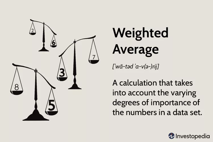
A deterministic, role-weighted Bayesian anchor where submissions are prioritized based on verified domain familiarity and historical editorial accuracy. Method 1 is the only pipeline that is role-aware: it models the assumption that trusted roles carry useful prior information about what kind of game a title is — especially when the population is still sparse.

The roles & base weights

The normative base weights are institutional authority parameters — they are not probabilities, not empirical accuracy estimates, and not effective sample sizes:

Role	Base weight	Weight symbol
Community	0.20	$w_g$
Community Leader	0.65	$w_g$
Moderator	0.95	$w_g$
Superuser / Staff	1.00	$w_g$

The anchor & population influence

Beyond the role weighting, Method 1 maintains a protected anchor — a hand-selected set of authoritative submissions treated as ground-truth anchors during catalogue bootstrapping. For $N \le 400$ the anchor is a raw equal average of its submissions; from $N \ge 401$ it switches to evidence-weighted averaging governed by the aggregate anchor reliability $\rho_A$ . The ordinary role weight $w_g$ is scaled by a population-influence coefficient $c(N)$ :

Very low population ( $N < 6$ ): the effective weight $q_g = w_g\,c(N) = 0$ , so the result is exactly the selected anchor average ( $F = A$ ). If no anchor qualifies, the calculation returns INSUFFICIENT_ANCHOR instead of fabricating a score.
Early growth ( $6 \le N < 9$ ): population influence turns positive, but the internal filters do not reject anyone — every submission receives $u_i = 1$ .
Filters engage ( $N \ge 9$ ): both complementary detectors become active — Method 1A, a mean- and SD-based absolute threshold with a 5-point floor, and Method 1B, a robust median-based threshold ( $3.5\,S_n$ ). Their verdicts weight each submission: $u_i = 1.0$ when both retain, $0.5$ when they split, and $0.0$ when both reject. Anchor submissions are never removed by these flags — detector disagreement reduces ordinary-role influence, not anchor membership.
Community fallback ( $N \ge 50$ ): when no privileged anchor exists, a Community fallback becomes available with a capped influence of $0.30$ .

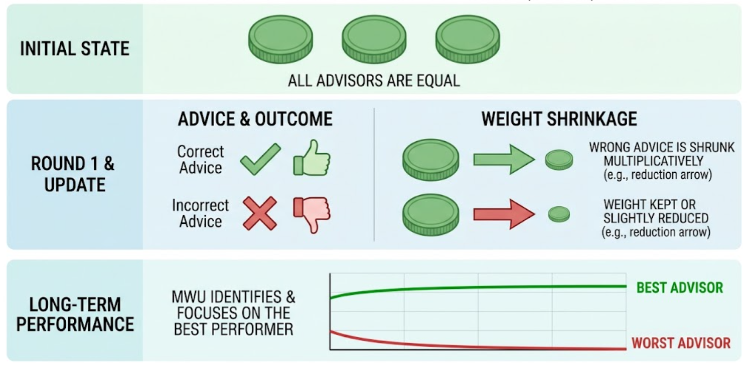
Method 1 solves the cold-start problem when a game has few submissions ( $N < 10$ ): with the statistical engines dormant, the anchored prior is the entire calculation, and the low- $N$ result is deliberately the anchor average rather than a noisy arithmetic mean. As the expert base expands, this system evolves toward the Multiplicative Weights Update Method (MWUM), dynamically penalizing inaccurate predictions and rewarding consistent calibration — and at high $N$ , statistically unsupported anchor submissions remain represented but are diluted rather than removed.

Learn more about Multiplicative Weights Update Method (MWUM)

Isolation Forest: anomalous data points isolated with fewer random partitions

2. Method 2 — Global Population Filtering

Isolation Forest (iForest)

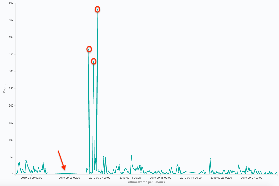
An unsupervised anomaly detection model that isolates global outliers across the six scalar dimensions without assuming normal distributions. It is not a density model, it is not role-aware, and it performs no cross-dimension standardization — each of the six scalar columns is analyzed by its own one-dimensional forest: $t = 512$ isolation trees per dimension, each built on a subsample of $\psi = \min(256, N)$ submissions drawn without replacement, with every tree capped at height $\ell = \lceil \log_2 \psi \rceil$ .

How the anomaly score works

Each tree recursively splits the dimension at random orthogonal thresholds. Genuinely anomalous points are easy to isolate — they need only a few partitions before they sit alone — so the number of splits required to isolate an observation is itself the signal. Averaging the path length across the forest gives $\bar h_{id}$ , and the canonical anomaly score is:

s_{id} = 2^{-\bar h_{id} / c(\psi)}

Short average path (few splits needed) drives the score toward 1 — the signature of an easily isolated, anomalous value.
A score near 0.5 means the observation's path length matches the expected reference depth for the subsample size $c(\psi)$ — a completely ordinary value.
Scores below 0.5 indicate deeper-than-expected isolation, i.e. values buried inside a dense region.

Flagging rule & the 2-of-6 rejection

A submission is flagged in a dimension only when $s_{id} > 0.60$ — strictly greater-than, so a score of exactly 0.60 is retained. The rule never selects a fixed percentage of observations: there is no contamination quota or forced rejection rate, and the number of flags may be zero, one, many, or all, depending purely on the data. A single flagged dimension is treated as a hint rather than a verdict; it takes flags in at least 2 of the 6 dimensions to reject the entire submission. Every survivor then carries equal weight (1.0) downstream — iForest prunes, it does not down-rank. Because the whole run is seeded (seed = 42), identical input populations reproduce identical flags within a calculation version.

Method 2 protects the dataset against chaotic haymakers, griefers, troll submissions, and bad-faith single-dimension flooding (e.g., scoring a tactical game as 100/0/0 Micro out of spite). What it cannot see is local context: a value that is globally unusual but coherent within its own small cluster can be swept up with the noise, which is exactly the failure mode Method 3 exists to correct.

Learn more about Isolation Forest

LoOP: a local density-based outlier diagram showing a point that clashes with its immediate neighborhood

3. Method 3 — Global Population Density

Local Outlier Probabilities (LoOP)

A local density-based statistical filter that asks a different question than iForest: not "is this value easy to isolate globally?" but "is this value's local spread unusually large compared to the spread of its own neighbors?" It runs independently on each of the six scalar dimensions using the absolute distance $d = |x - y|$ , a tie-inclusive $k = 10$ nearest-neighbor neighborhood, and a standard-deviation extent $\lambda = 3$ . Tie-inclusion matters because submissions are integers on a bounded 0–100 scale — exact ties are common and must not be discarded.

From local distance to a probability

Each submission gets a probabilistic distance $\text{pdist}_i = \lambda \sigma_i$ — its neighborhood's spread scaled by the extent parameter — and the neighborhood reference $\overline{\text{pdist}}_i$ , the mean of its neighbors' probabilistic distances. The ratio of the two yields the Probabilistic Local Outlier Factor, the relative excess local spread around the submission:

\text{PLOF}_i = \frac{\text{pdist}_i}{\overline{\text{pdist}}_i} - 1

A positive $\text{PLOF}_i$ means the submission has greater local spread than its neighbors; zero means it matches the neighborhood reference; a negative value means it sits in a locally denser region. Raw PLOF values are normalized across the population by the root-mean-square factor $n\text{PLOF} = \lambda \sqrt{\frac{\sum_{i \in \mathcal{F}} \text{PLOF}_i^2}{|\mathcal{F}|}}$ and mapped into $[0, 1]$ through the Gauss error function:

\text{LoOP}_i = \max\left[0,\ \operatorname{erf}\left(\frac{\text{PLOF}_i}{n\text{PLOF}\sqrt{2}}\right)\right], \qquad \operatorname{erf}(z) = \frac{2}{\sqrt{\pi}}\int_0^z e^{-t^2}\,dt

A submission is flagged only when $\text{LoOP}_i > 0.75$ — strictly greater-than, so a probability of exactly 0.75 is retained — and the same universal 2-of-6 rejection rule applies across the six dimensions. The LoOP probability is a relative anomaly measure: it ranks how atypical a submission looks within its neighborhood. It is not a posterior probability that a submitter is wrong or malicious — outlier status means statistical atypicality under this detector, and nothing more.

How it differs from iForest

iForest analogy: Spotting a lone skyscraper in the middle of open farmland — an obvious global outlier.
LoOP analogy: Spotting a single suburban single-family home placed inside dense downtown Manhattan — it looks normal in isolation, but completely clashes with the density of its immediate neighbors.

Method 3 captures subtle sub-population disagreements that global methods cannot see. If a cluster of players agrees a game is Mystiko-heavy but a sub-cluster scores it as pure Macro within an otherwise cohesive local group, LoOP measures the local reachability density and downweights the anomalous local cluster — while preserving a globally distant but internally dense subgroup, which iForest would have pruned as noise.

Learn more about Local Outlier Factor (LOF) & LoOP

How We Aggregate Submissions to Compute the Final Score

Three pipelines run on every classification epoch. They never run in isolation: Method 1 anchors the prior, while Methods 2 and 3 clean the population before the final consolidation step.

Each contributing player submits two independent profiles — a Challenge profile (what the game demands) and a Reward profile (what the game returns) — each split across Micro, Macro, and Mystiko and normalized so the three components of every profile sum to 100. A single epoch therefore presents the pipeline with six scalar columns of data: $C_\mu,\ C_M,\ C_Y,\ R_\mu,\ R_M,\ R_Y$ . All three methods analyze those six columns independently — none of the detectors ever sees the composition as a single joint object.

Each method $\mathcal{M}_k$ returns a continuous six-component result — a Challenge triple and a Reward triple, each summing exactly to 100:

\mathcal{M}_k(D) = \left(\mathbf{m}_{kC}, \mathbf{m}_{kR}\right), \qquad \sum_j m_{ktj} = 100

These are continuous pre-reconciliation outputs. The unification layer consumes the continuous values — never the rounded integers — and only the final published profile is reconciled to whole numbers. Method 1 contributes the expertise-sensitive perspective $\mathbf{E}_t$ , Method 2 the globally robust population perspective $\mathbf{G}_t$ , and Method 3 the locally robust population perspective $\mathbf{L}_t$ — three independent answers to the same question, consolidated by BHPCM at the end.

Architectural & Statistical Deep Dives

Why employ two different methods of removing outliers?

iForest strengths: Efficient at catching wild, non-linear global outliers — 512 trees per dimension over a $\min(256, N)$ subsample, with no pairwise distance calculations at all.
iForest weaknesses: Blind to local density variation; a small but legitimate consensus cluster that sits far from the global mass can be pruned as if it were noise. Its binary flag ( $s_{id} > 0.60$ strict) says nothing about how far past the threshold an observation lies.
LoOP strengths: Produces a mathematically calibrated probability score $[0, 1]$ from local neighborhood density (tie-inclusive $k = 10$ , extent $\lambda = 3$ ), so a niche playstyle that is coherent within its own neighborhood survives even when it differs from the global majority.
LoOP weaknesses: Computationally intensive ( $O(N^2)$ pairwise distance checks) and sensitive to the neighborhood size $k$ . Its flag is also strictly greater-than ( $\text{LoOP}_i > 0.75$ ), and a LoOP probability is a relative anomaly measure, not a posterior probability that a submitter is wrong.

The reality of data & hardware: combining global tree-based isolation with local density probabilities ensures the platform is protected against malicious vandalism without erasing genuine subjective nuance. Disagreement between the two engines is analytically useful rather than a bug — it can reveal expert/population tension, a coherent minority playstyle, globally isolated observations, locally sparse observations, heavy ties, or multi-modal submission behavior. Neither engine is a popularity vote, and neither engine can unilaterally decide a classification — each only prunes submissions before the BHPCM consolidation stage.

In what scenarios would Method 1 ever "beat" Methods 2 and 3 in reliability?

The cold-start trap: Methods 2 and 3 are only invoked once a population reaches $N \geq 20$ ; below that threshold the statistical engines are dormant and the anchored prior is the entire calculation. Even in the 20–50 range, small samples lack the statistical power to distinguish a genuine niche opinion from an anomaly, so outlier rejection can misclassify valid minority viewpoints. Method 1's internal filters also calibrate earlier — its detectors switch on at $N \geq 9$ , while iForest and LoOP need $N \geq 20$ .
Expert calibration: In early classification epochs, a single verified expert submission anchored via Method 1 provides a mathematically grounded baseline that prevents uncalibrated public sentiment from skewing the initial index. As N grows, the anchor's influence is diluted rather than removed — it remains represented but ceases to dominate, and the system transitions smoothly from expert-led to community-led governance.

Why is "Superuser" even a role in Method 1?

Operational checks & balances: Serves strictly as a bootstrapping mechanism to establish ground-truth anchors across initial catalogue releases. A Superuser classification is a calibration anchor, not a veto.
Classification ≠ quality judgments: MyGameDNA measures what kind of game a title is, not whether it is good or bad. A Superuser bias has zero moral or commercial impact on review aggregates — it merely anchors mechanical categorization.
Pledge of impartiality: Staff classifications pledge strict adherence to observable mechanical inputs. As the contributor and expert dataset matures, the Superuser weighting phase-out is baked into the convergence algorithm. The base-weight table above makes the institutional authority explicit — a normative governance choice, not a hidden empirical claim. Feedback is continuously welcome.

How are the three methods consolidated into a single score?

Bayesian Hierarchical Pluralistic Consensus Model (BHPCM): rather than computing an arithmetic mean (which is vulnerable to residual skew), BHPCM treats a skill profile as a composition and works in isometric log-ratio (ilr / Aitchison) geometry: the six components are embedded in a five-dimensional log-ratio space, and distances between profiles are measured with the Aitchison distance — never Euclidean distance on raw percentages, which would let scale artifacts dominate the comparison. All probabilistic combination, covariance estimation, disagreement measurement, and posterior averaging happens in this space.

Method 1 supplies the expertise-sensitive prior ( $\mathbf{E}_t$ ); Methods 2 and 3 provide the cleaned population likelihood — the globally robust ( $\mathbf{G}_t$ ) and locally robust ( $\mathbf{L}_t$ ) perspectives. The two population perspectives are treated as correlated — they consume the same submissions, so their outputs must not be pooled as independent votes. A stratified bootstrap resamples the submission population to propagate uncertainty through both perspectives, and the posterior distribution of the governed compromise yields the unified score plus a mathematical Confidence Level.

Why BHPCM beats simple or weighted averages:

Variance shrinkage: Automatically pulls extreme scores toward the consensus mean when sample variance is high.
Dynamic uncertainty weighting: The influence of the expertise perspective is bounded by explicit governance parameters — a permitted minimum and maximum. If Methods 2 and 3 show high inter-method agreement, the model reduces the prior's influence toward its minimum, transitioning smoothly from expert-led to community-led governance; strong expert–population disagreement similarly tamps the expert anchor down rather than letting either side win by default.
Pluralism without averaging: Disagreement is treated as legitimate diversity of judgment, not as evidence that one side is objectively wrong — BHPCM never assumes a single objectively correct score vector. Disagreement is preserved in the uncertainty, not repaired away.
Integer reconciliation: The posterior is a continuous composition; the published profile is recovered by largest-remainder allocation so each profile sums to exactly 100, with a fixed tie priority (Micro wins a 0.5/0.5 Micro–Mystiko remainder tie).